start of lec 19
This lecture we will learn about periodic functions, specifically, non-sinusoidal periodic functions.
Periodic function
Definition:
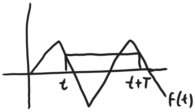
$f$ is periodic with period $T \quad (T>0)$ if:
$$f(t)=f(t+T), \quad \forall\ t\in \mathbb{R}$$
We will now compute laplace transforms of these periodic functions. Computing DE's containing these periodic functions using something like voparam would not be easy.
Let's try taking the laplace of a periodic function $f(t)$:
If we take the windowed version of the function (one period, where everywhere else is 0, ie:)
$f_{T}(t)=\begin{cases}f(t)\ ,\ & 0\leq t\leq T \\\\0\ ,\ & \text{otherwise}\end{cases}$
we can "glue together" many of these windows together to rebuild our $f(t)$, like this:
$f(t)=f_{T}(t)+f_{T}(t-T)+f_{T}(t-2T)+\dots$
We can add some unit step functions strategically such that it doesn't change the overall expression:
$f(t)=f_{T}(t)+f_{T}(t-T)u(t-T)+f_{T}(t-2T)u(t-2T)+\dots$
hit it with the LT!
$\mathcal{L}\{f\}=\mathcal{L}\{f_{T}\}+\mathcal{L}\{f_{T}(t-T)u(t-T)\}+\dots$
recall the formula from last lec: $\mathcal{L}\{u(t-a)f(t-a)\}=e^{-as}F(s)$
then:
$\mathcal{L}\{f\}=\mathcal{L}\{f_{T}\}(1+e^{-Ts}+e^{-2Ts}+e^{-3Ts}+\dots)$
$\mathcal{L}\{f\}=\mathcal{L}\{f_{T}\}(1+e^{-Ts}+(e^{-Ts})^{2}+(e^{-Ts})^{3}+\dots)$
This is a geometric series! $1+r+r^2+\dots$
Geometric series are convergent when $|r|<1$
and equal to: $\frac{1}{1-r}$
in this case, $r=e^{-Ts}$
so:
$$\mathcal{L}\{f\}=\mathcal{L}\{f_{T}\} \frac{1}{1-e^{-Ts}}$$
handy formula! ^ will be used again.
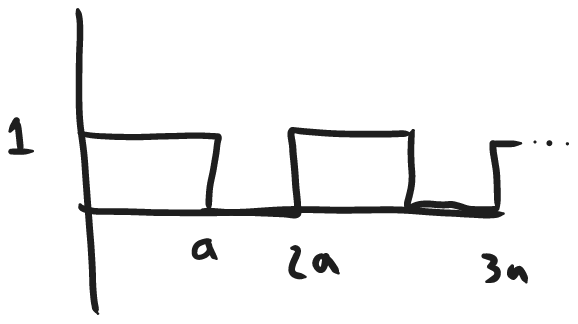
Imagine another function: (image is of a square wave with a period of 2a, oscillates between 1 and 0, starts at 1 when t=0.)
Let's compute its LT:
$\mathcal{L}\{f\}=\mathcal{L}\{f_{2a}\} \frac{1}{1-e^{-2as}}$
$f_{2a}=u(t)-u(t-a)$ (this is the first period piece)
$\implies \mathcal{L}\{f_{2a}\}=\mathcal{L}\{u(t)\}-\mathcal{L}\{u(t-a)\}=\frac{1}{s}- \frac{e^{-as}}{s}$
plug back in:
$\mathcal{L}\{f\}=\mathcal{L}\{f_{2a}\} \frac{1}{1-e^{-2as}}=\frac{1}{s}\cancel{ (1-e^{-as}) } \frac{1}{\cancel{ (1-e^{-as}) }(1+e^{-as})}$
$$\mathcal{L}\{f\}=\frac{1}{s(1+e^{-as})}$$
ex IVP periodic second_order_nonhomogenous LT partial_fractions
Solve for $y(t)$ in the following second order periodic equation:
$$y''+3y'+2y=f(t) \qquad y(0)=y'(0)=0 \quad a=1$$where $f(t)$ is from the previous example and $a$ is the width of $\frac{1}{2}$ of a period in the function $f(t)$. This means $f(t)$ has a period of $T=2$
Hit it with the LT!
$s^2Y+3sY+2Y=\mathcal{L}\{f\}= \frac{1}{s(1+e^{-1s})}$
$(s+1)(s+2)Y= \frac{1}{s(1+e^{-1s})}$
$Y(s)=\frac{1}{s(s+1)(s+2)} \frac{1}{1+e^{-s}}$
What property can we use to find the inverse of that?
psst. We can use $\mathcal{L}\{y\}=\mathcal{L}\{y_{T}\} \frac{1}{1-e^{-Ts}}$ ;)
$Y(s)=Y_{T}(s) \frac{1}{1+e^{-s}}$ But this is not true! because:
That second term has a $1+e^{-Ts}$ term in the denominator, it doesn't match up in the formula. There is a fix, peep this:
$Y(s)=Y_{T}(s) \frac{1-e^{-s}}{(1+e^{-s})(1-e^{-s})}$
$Y(s)=Y_{T}(s) \frac{1-e^{-s}}{1-e^{-2s}}$ We are rather lucky, the 2 in the denominator matches $T$, the period of our function.
We can tuck away the numerator into $Y_{T}(s)$ (this does redefine $Y_{T}$ to the correct expression, and the equation below is now true.)
$Y(s)=\underbrace{ \frac{1-e^{-s}}{s(s+1)(s+2)} }_{ Y_{T}(s) } \frac{1}{1-e^{-2s}}$
Our equation is now in the correct form. We can now calculate the inverse of $Y_{T}(s)$
Split up $Y_{T}(s)$ :
$Y(s)= \underbrace{ (\frac{1}{s(s+1)(s+2)} }_{ F_{1}(s) }-\underbrace{ \frac{e^{-s}}{s(s+1)(s+2)} )}_{F_{2}(s) } \frac{1}{1-e^{-2s}}$
We can use partial fractions for the first term and
$\mathcal{L}\{u(t-a)f_{1}(t-a)\}=e^{-as}F_{1}(s)$ for the second term. (Where $a=1$)
Using partial fractions:
$\frac{1}{s(s+1)(s+2)}=\frac{A}{s}+\frac{B}{s+1}+\frac{C}{s+2}$
$A(s+1)(s+2)+Bs(s+2)+Cs(s+1)=(A+B+C)s^2+(3A+2B+C)s+2A=1$
$2A=1\implies A=\frac{1}{2}$
$\frac{3}{2}+2B+C=0$
$\frac{1}{2}+B+C=0$
subtract the two equations.
$1+B=0\implies B=-1$
$\implies C=\frac{1}{2}$
$\mathcal{L}^{-1}\{F_{1}\}=\mathcal{L}^{-1}\{\frac{1}{2} \frac{1}{s}-\frac{1}{s+1}+\frac{1}{2} \frac{1}{s+2}\}$
$\mathcal{L}^{-1}\{F_{1}\}=f_{1}(t)=\frac{1}{2}-e^{-t}+\frac{1}{2}e^{-2t}$
Second term, $F_{2}(s)$, use: $\mathcal{L}\{u(t-a)f_{1}(t-a)\}=e^{-as}F_{1}(s)=F_{2}(s)$
$f_{2}(t)=u(t-1)(\frac{1}{2}-e^{-(t-1)}+\frac{1}{2}e^{-2(t-1)})$
recombine the two parts:
$Y_{T}=F_{1}-F_{2}$
$\mathcal{L}^{-1}\{Y_{T}\}=\mathcal{L}^{-1}\{F_{1}\}-\mathcal{L}^{-1}\{F_{2}\}$
$y_{T}(t)=f_{1}(t)-f_{2}(t)$
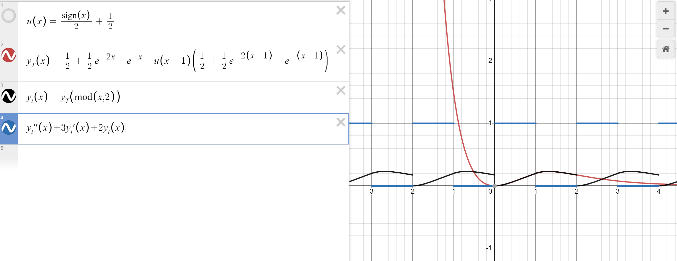
$y(t)$ is a periodic function, with period of $T=2$
It's windowed form, $y_{T}$, is:
$$y_{T}(t)=\frac{1}{2}+\frac{1}{2}e^{-2t}-e^{-t}-u(t-1)(\frac{1}{2}-e^{-(t-1)}+\frac{1}{2}e^{-2(t-1)})$$
Peep da plot!